FISSION TRACK DATING METHODS

Evaluating a fission track age

The fission track age equation

The fission track age equation is a specialised form of the general age equation used in all other forms of radiometric dating. In this case the ratio of atoms which have undergone radioactive decay to the number of parent atoms remaining is expressed by the ratio of spontaneous to induced track densities (Price and Walker 1963, Naeser 1967):

$$\large t = { 1 \over \lambda_D } \ln \left ( 1 + {\lambda_D \phi \sigma I \over \lambda_f} {\rho_s \over \rho_i } \right ) \qquad \qquad \large 1 $$

where:

• \(\lambda_D \) = total decay constant for \(^{238}U, 1.55125 \times 10^{-10}yr^{-1}\)
• \(\lambda_f \) = spontaneous fission decay constant of \(^{238}U\)
• \(I\) = isotopic ratio \(^{235}U\)/\(^{238}U \), 7.2527x10\(^{-3} \)
• \( \sigma \) = thermal neutron cross-section for \( ^{235}U, 580.2 \times 10^{-24}cm^{-2}\)
• \(\phi \) = thermal neutron fluence
• \(\rho_s \) = spontaneous track density
• \(\rho_i \) = induced track density

It is important to note that the use of equation (1) to calculate a fission track ages assumes that all grains have the same fission-track age and that that variation between them is due to the Poissonian distribution of the track counts. Since the values of the constants \(I, \lambda_D\), and \(\sigma \) are well known, only the two track densities, \(\rho_s\) and \(\rho_i\), the neutron fluence \(\phi\), and the decay constant \(\lambda_f \), are required to evaluate the age \(t\). The two track densities are determined from the numbers of tracks counted (\(N\)) divided by the area (\(A\)) counted for both spontaneous and induced tracks where:

$$ \large \rho_s = { N_s \over A } \ \qquad and \qquad \rho_i = { N_i \over A }$$

The systematics and calibrations involved in calculating a fission track age via equation (1) have been extensively reviewed by Hurford and Green (1982) and Wagner and van den Haute (1992). Usually two or more standard glass/mica dosimeters are included in each irradiation package to monitor the neutron fluence, and any gradient it might have along the package. After irradiation the tracks are etched in the mica and counted, as described above. The glass can be reused many times as only a tiny fraction of the uranium (about \(10^{-6} \)) is used up in a typical fission track irradiation. The fluence is directly related to the track density in the mica, \( \rho_d \), by:

$$ \large \phi = B \rho_d \qquad \qquad 2$$

where the constant \(B\) is a calibration factor. The value of \(B\) is often determined against independent activation foil measurements of the fluence, or by reference to fission track dating of an age standard using an assumed value of \( \lambda_f \). However, there have been significant difficulties in determining the neutron fluence received by an irradiation package under different reactor conditions and in the independent determination of the spontaneous fission decay constant, \(\lambda_f\), for \(^{238}U\).

5.2 Calibration

The value of the spontaneous fission decay constant for \(^{238}U\) was disputed for many years and the controversy was reviewed by Fleischer et al., (1975), Bigazzi (1981), Hurford and Green (1981), (1982), (1983) and Wagner and van den Haute (1992). Fission track dating studies have tended to use values close to either \(7.03\times10^{-17} yr^{-1} \) or \( 8.42\times10^{-17} yr^{-1} \). The difference between these two values is about 20%, vastly greater than their quoted uncertainties of around 1%. Successive determinations of the decay constant over recent years have tended to cluster around one or other of these two values and there seems no prospect of an early resolution to this ambiguity.

Experience in numerous fission track dating laboratories has shown that neutron dosimetry using activation foils can also be extremely unreliable. The theoretical background and practical application of neutron dosimetry techniques have been discussed in detail by Green and Hurford (1984). The reproducibility of fluence calibrations between different laboratories has proved to be about as poor as that for the spontaneous fission decay constant. It has been pointed out by Hurford and Green (1982) that this is by no means coincidental, as in many cases the determinations of the decay constant have depended on fluence measurements. These authors concluded that any value of \(\lambda_f\) calculated using a system of thermal neutron dosimetry will only be valid for that particular system.

Despite this degree of uncertainty, it is clear that fission track measurements on age standards can give reproducible results, and that these can be in close agreement with the independent age using various combinations of \('\lambda_f'\) and \('B'\). Much of the argument over decay constants has thus, in reality, been about the selection of suitable calibration factors. If an overall calibration is carried out against age standards, then in essence what is derived is a calibration ratio (\(B/ \lambda_f \)) which is often split into the two notional components, often quite arbitrarily. It must be accepted that, at present, the absolute values of these two components are simply not known independently of each other. Until such time as independent measurements of \(B\) and \( \lambda_f\) are obtained which are widely agreed to be precise and free of any possibility of significant systematic error, fission track dating will continue to be a system which must be empirically calibrated against independently known ages, principally from K- Ar and \(^{40}Ar/^{39}Ar\) dating.

Hurford and Green (1982, 1983) and Hurford (1990a,b ) have argued strongly in favour of a direct empirical calibration of the age equation, as first suggested by Fleischer and Hart (1972). If we substitute equation (2) into equation (1) we get:

$$ \large t = { 1 \over \lambda_D } \ln \left [ 1 + {\rho_s \over \rho_i} \sigma I \lambda_D \left ( {B \rho_d \over \lambda_f } \right ) \right ] \qquad \qquad \large 3 $$

All of the constants in (3), except for \(\lambda_D\) which effectively cancels out of the equation for young ages (<100 Ma), can be taken together as a single factor, zeta (\(\zeta \)), which can be calibrated directly by reference to age standards. Equation (3) then becomes:

$$ \large t = { 1 \over \lambda_D } \ln \left ( 1 + \lambda_D \zeta {\rho_s \over \rho_i} \rho_d \right ) \qquad \qquad \large 4 $$

The value of the zeta factor will be specific for a particular standard glass and can be evaluated from fission track determinations on age standards by:

$$ \large \zeta = { ( e^{\lambda_Dt_{std}} - 1 ) \over \lambda_d \left ( {\rho_s \over \rho_i} \right )_{std} \rho_d } \qquad \qquad \large 5 $$

which is equivalent to \( \sigma I B \over \lambda_f\), but can be determined empirically .

The empirical zeta calibration factor must be calculated for each fission track worker and should be averaged over many separate determinations. Typically each fission track measurement will be made between 5 and 10 times on each age standard and then averaged to give the final zeta value. Ideally, the repeat measurements should include a number of different irradiations. Ratios of counts obtained using various standard dosimeter glasses in common use have been given by Hurford and Green (1983), which can be used to compare zeta factors obtained with one dosimeter glass to those obtained with another.

It is important that such a system calibration be based on a series of measurements on age standards and not on a single determination, which can be far less precise. Obviously the selection of materials for use as age standards is crucial to the success of the overall calibration. The requirements which must be met by any potential standard are given by Hurford and Green (1983). Suitable standard materials are rare and so far the most successful have been apatite and zircon from the Fish Canyon Tuff, an extensive ignimbrite unit in southern Colorado (Naeser et al. 1981). Suitable apatite and sphene have also been obtained from a sub-volcanic intrusion in the Mt Dromedary Complex of southern N.S.W. The apatite from Cerro de Mercado, Durango. Mexico is also routinely used as a standard.

5.3 Age Equation for the LA-ICP-MS Method

Where the uranium 238 concentration of a mineral grain is determined explicitly using LA-ICP-MS (see section 3.5), equation 4 above is modified to:

$$ \large t = { 1 \over \lambda_D } \ln \left ( 1 + \xi {\rho_s \over C_u} \right ) \qquad \qquad \large 6 $$

$$ \large where $$

$$ \large \xi = {\lambda_D A \over \lambda_f N_0 D R \alpha} \qquad \qquad \qquad 7 $$

and:

• \(C_u\) = concentration of \(^{238}U\)
• \(A\) = atomic weight of \(^{238}U\)
• \(N_0\) = Avogadro’s Number
• \(D\) = denisty of the mineral
• \(R\) = etchable range of one fission fragments (= half confined track length, 8.1 μm)
• \(\alpha\) = detection efficiency for the etched surface).

In practice the constant \(\xi\) (Xi) can be measured empirically against a set of age standards, as for the Zeta approach. However, all of the constituents constants are known to varying degrees, raising the possibility to a return to an absolute calibration of fission track ages. More experimental work is required to fully asses the values of all of these constants.

5.4 Estimation of Uncertainty

The statistical analysis used in fission track dating has received considerable discussion in the literature (e.g. Green 1981, Galbraith & Laslett, 1993, Galbraith, 2005 and references therein). The fundamental assumption of fission track statistics is that track counts, like radioactive decays, will follow a poisson distribution. The so-called conventional analysis of errors assumes that no further sources of variation are present in the measurement of track densities. For a poisson distribution the standard deviation, \(s\), of a track count is given by the square root of the total number of tracks counted, \(N\):

$$ \large s = \sqrt{N} \qquad \qquad \large 8 $$

A standard deviation can be assigned in this way to each track density measurement used in calculating a fission track age. These errors are combined to give the standard deviation of the age, \(s_t\), as follows

$$ \large s_{t} = \sqrt{{1 \over N_{s}} + {1 \over N_{i}} + {1 \over N_{d}} + \left ( {s_{\zeta} \over \zeta } \right )^{2} } \qquad \qquad \large 9 $$

where \(N_s\), \(N_i\) and \(N_d\) are the total number of tracks counted for spontaneous, induced and standard glass track densities, respectively, and \(s_\zeta\) is the standard deviation of the empirical determination of the calibration constant \( \zeta\).

Other, non-poissonian, sources of variation are in fact possible (e.g. Green 1981) so that the conventional analysis in equation (9) is actually a limiting best case. Galbraith (1982) has described a \( \chi^2\) test which can be used to test whether variation is present in excess of that predicted from poisson statistics (see 5.4 below). Experience has shown, however, that the great majority of results obtained by the external detector method, on materials such as age standards, pass the \( \chi^2\) test indicating that the assumption of poisson variation is often reasonable for this method.

The same analysis is often applied to results obtained by the population method, but this will be valid only in the limiting case where the uranium concentration of all grains is the same. Where there is variation in uranium between grains, which is likely in most cases, then the uncertainty calculated from equation (9) will be an underestimate. No rigorous treatment of error estimation has yet been made for the population method, and errors are usually calculated from the standard deviations of the actual grain counts, assuming them to be normally distributed. The combined error is calculated from:

$$ \large s_{t} = t \sqrt{ { \left ( \bar{s} \over \bar{x} \right ) ^ {2} _s } + {\left ( \bar{s} \over \bar{x} \right ) ^ {2} _i } + { 1 \over N_{d}} + { \left ( s_{\zeta} \over \zeta \right )^{2} } } \qquad \qquad \qquad 10 \large $$

where s is the standard error of the mean (i.e. \( s \over \sqrt {N } \) ) for the raw grain counts, and \( \bar x \) is the mean count. Subscripts s and i indicate spontaneous and induced tracks respectively. The contribution to the error from the standard glass count, \( N_{d} \), is taken to be the poisson error as before.

When reporting fission track results it is important that all the analytical data and all constants used in calculating the age and error are quoted. A recommended format for fission track data reports has been outlined by Naeser et al. (1979), which aims at ensuring sufficient information is given to adequately evaluate an age determination. Further pertinent comments in this regard are given by Hurford and Green (1982).

5.5 Assessing variation between single-grain ages

The discussion so far has been based on the assumption that there is no variation in the calculated fission track ages of single grains beyond that expected from the Poissonian distribution of the fission track counts. The external detector method is important for testing this assumption in that it allows the determination of \( \rho_{s}/\rho_{i}\) for individual crystals, as discussed in Gleadow and Lovering (1977), Gleadow (1981) and Hurford and Green (1982). The ability to calculate individual grain ages is vital in assessing whether the range of ages present reflect a single population or multiple age populations. The presence of multiple populations is of course critical in the interpretation of fission track ages (Gleadow and Duddy, 1981, Green et al., 1985, 1986, 1989, Crowley et al., 1991, Carlson and Donelick, 1993, O’Sullivan and Parrish, 1995). An objective test of whether there is real variation in single grain ages beyond that expected from the track counts alone can be obtained from the determination of a \( \chi ^{2}\)) statistic (Green, 1981).

$$ \large \chi^{2} = {\sum^{n} _{j=1} } {\left ( N_{sj} - \bar N_{sj} \right )^{2} \over \bar N_{sj} } + {\sum^{n} _{j=1} } { \left ( N_{ij} - \bar N_{ij} \right )^{2} \over \bar N_{ij} } \qquad \qquad \large 11 $$

where:

$$ \large \bar N_{sj} = {N_{s} \over N_{s} + N_{i}} \left ( N_{sj} + N_{ij} \right ) $$

$$ \large \bar N_{ij} = {N_{i} \over N_{s} + N_{i}} \left ( N_{sj} + N_{ij} \right ) $$

If the \(\chi^{2}\) probability (\(P\chi^{2}\)) value is >5% then the single grain ages determined can be considered to approximate a normal Poissonian distribution (Green 1981) In this case it is valid to calculate the ratio \(\rho_{s}/\rho_{i}\) using the sum of track counts (pooled age) from all grains counted (see equations 12 and 13; the age is calculated by substituting equations 10 and 11 in to equation 4). It is important to note that a pooled age assumes that all grains are related to a single age and fit within a Poissonian distribution.

$$ \large \rho = { {{\sum^{n} _{j=1} } N_{sj}} \over { { {\sum^{n}_{j=1} } A_{sj} } } } \qquad \qquad \large 12 $$

>$$ \large \rho = { {{\sum^{n} _{j=1} } N_{ij}} \over { { {\sum^{n}_{j=1} } A_{ij} } } } \qquad \qquad \large 13 $$

If the value of \(P\chi^{2}\) is <5% the range in single grain ages or variation in \(\rho_{s}/\rho_{i}\), will be greater than expected for a Poissonian distribution. In this case the assumption made in the calculation of a pooled age, that the grains belong to a single population, is not valid. To overcome this problem, calculation of a mean age was suggested by Green (1981). When calculating a mean age the ratio of \(\rho_{s}/\rho_{i}\) required in equation 4 is equal to the sum of the individual \(\rho_{s}/\rho_{i}\) values divided by the number of grains (equation 14, \(\rho_{s}\) and \(\rho_{i}\) values are calculated for each individual grain, j). The mean age is thus given by:

$$ \large {\left [ {\rho_{s} \over \rho_{i} } \right ]} = {{\sum^{n} _{j=1} } {{\left [ {\rho_{s} \over \rho_{i} } \right ] _{j}} \over n }} \qquad \qquad \large 14 $$

Although the mean age is more valid than the pooled age at \(P\chi^{2}\) values of <5%, it only depends on the ratio of \(N_{s}/N_{i} \) and not on the magnitude of the individual track counts (Galbraith and Laslett, 1993). As a result the mean age gives equal weight to each individual grain and will give undue influence to grains that have very small track counts.

5.6 The Central Age

Galbraith and Laslett (1993) introduced the Central Age as a more accurate assessment of age variation in samples having \(P\chi^{2}\) values <5%, as well as for samples that represent a single age population. The central age is the population geometric age, which has a standard deviation (i.e. age dispersion) which can be estimated. Calculation of the central age and dispersion is less straightforward to calculate, however, and is most easily determined iteration of the following algorithm given by Galbraith and Laslett (1993, Appendix A2):

\( 1.\space for \space j = 1,2,...,n \space let \)

$$ \large m_{j} = N_{sj} + N_{ij} $$

$$ \large y_{j} = { N_{sj} \over m_{j} } $$

$$ \large z_{j} = log \left ( { N_{sj} + 1/2 \over N_{ij} + 1/2} \right ) $$

\( 2. \space Set \space initial \space values \space for \space \sigma \space and \space \eta. \space For \space example: \)

$$ \large \sigma = 0.6 \times \space standard \space deviation \space of \space \left \{ z ,z ,...,z \right \} $$

$$ \large \eta = {{\sum^{n}_{j=1}} N_{sj} \over {\sum^{n}_{j=1}} m_{j}} $$

\( 3. \space For \space j = 1,2,...,n \space compute \)

$$ \large w_{j} = { m_{j} \over \left \{ \eta \left ( 1 - \eta \right ) + \left (m_{j} - 1 \right )\eta^{2}\left ( 1 - \eta\right )^{2} \sigma^{2} \right \} } $$

\( 4. \space Compute \space new \space values \space of \space \sigma \space and \space \eta \space as \)

$$ \large \sigma = \sigma \left ( { {\sum^{n}_{j=1} w ^{2}_j} { \left( y_{j} - \eta \right )^{2} } } \over { {\sum^{n}_{j=1} w _j} } \right ) $$

$$ \large \eta = {\sum^{n}_{j=1} w _{j} y _{j} } \over {\sum^{n}_{j=1} w _{j}} $$

\( 5. \space Recalculate \space steps \space 3 \space and \space 4 \space until \space \sigma \space and \space \eta \space do \space not \space change, \)

\( \space which \space is \space usually \space achieved \space within \space 20 \space iterations \space (Galbraith \space and \space Laslett, \space 1993). \)

\( 6. \space The \space final \space value \space for \space \sigma \space is \space the \space estimate \space for \space the \space age \space dispersion \space and \space the \space final \space value \space for \space \eta \space is \)

\( substituted \space in \space the \space age \space equation \space (4) \space given \space the \space relationship: \)

$$ \large {\rho_{s} \over \rho_{i}} = {\eta \over \left ( \eta - 1 \right )} $$

\( so \space that \space the \space central \space age, t_{c}, \space is \space given \space by: \)

$$ \large t_{c} = {1 \over \lambda_{D}} \ln \left ( 1 + \lambda_D \zeta \rho_{d} { \eta \over {1 - \eta}} \right ) $$

\( and \space the \space age \space dispersion, \space s(t_{c}), \space by: \)

$$ \large s(t_{c}) = t_{c} \sqrt{{ 1 \over {\eta^{2} \left( 1 - \eta \right )^{2} {\sum^{n}_{j=1} w _{j}} } } + {1 \over N_{d}} + {\left ( s_{\zeta} \over \zeta \right) ^{2} } } $$

The central age and age dispersion are most readily calculated by means of a computer program which carries out the necessary iteration automatically (see 5.8 below).

5.7 Calculation of Uranium Concentration

Calculation of the uranium concentration for individual mineral grains is accomplished through reference to a dosimeter glass (such as SRM612 or CN5) of known uranium concentration. The uranium concentration of an unknown mineral grain can be calculated from the induced track density recorded in an external detector over that grain, \(\rho_{i}\), as shown in the following relationship.

$$ \large U_{unk} = {\rho_{i} \over \rho_{d} } U_{std} \qquad \qquad 17 $$

Where:

• \( U_{unk} \) = uranium concentration of unknown mineral grain
• \( \rho_{i} \) = induced track density over the grain
• \( \rho_{d} \) = induced track density in an external detector over the standard glass
• \( U_{std} \) = uranium concentration of the dosimeter glass (e.g. SRM-612, CN5).

5.8 Presentation of data

It is important that fission track analytical results are presented in a form that enables the results to be properly assessed and fully interpreted by the reader. The Subcommision on Geochronology of the International Union of Geological Sciences made detailed recommendations on system calibration and data reporting which are reported by Hurford (1990a, 1990b). These recommendations provide the basic template for all reporting of fission track age data and a modern example incorporating the central age is shown in Table 5.1.

Table 5.1:
Specimen table showing the presentation of fission track dating results

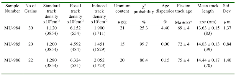
Brackets show number of tracks counted or measured. Standard and induced track densities measured on mica external detectors (g = 0.5) and fossil track densities on internal mica surfaces. All ages shown are central ages. se = standard error of the mean track length.
*Age calculated using zeta = 384±5 for Corning glass dosimeter CN-5.

Some aspects of fission track data are best shown graphically, such as the distribution of track lengths and radial plots of grain ages. Examples of these are shown in Figure 5.2. For a population of single grain ages the radial plot is the most effective way to visualise the precision and spread around the central age. The graphs shown in Figure 5.2 were generated as an output of the computer program MacTrack. Similar results are available from the package RadialPlotter (see links under 5.8 below).

On a radial plot, the age of a single mineral grain is found by extrapolating a line from the zero point through the grain point to the age axis on the right. The 2σ error for a grain is found by extrapolating lines from the zero point to the age axis passing through the standard error of the sample. The standard error is the same for all grains in a sample and is indicated on the y axis. The precision or relative error for each grain is indicated by the x axis. Grains that lie close to the y axis are less precise (have a larger relative error) than those that lie to the right. The radial plot allows the visual recognition of distinct populations in a sample (when \( P\chi^{2}\) is < 5%, or variation is high), excellent examples of which are seen in O’Sullivan and Parish (1995). The central age (central), \( \chi^{2}\) probabillity (\( P\chi^{2}\)) and variation (Var) are indicated on the right hand side of the radial plot to allow comparison with the graphical form.

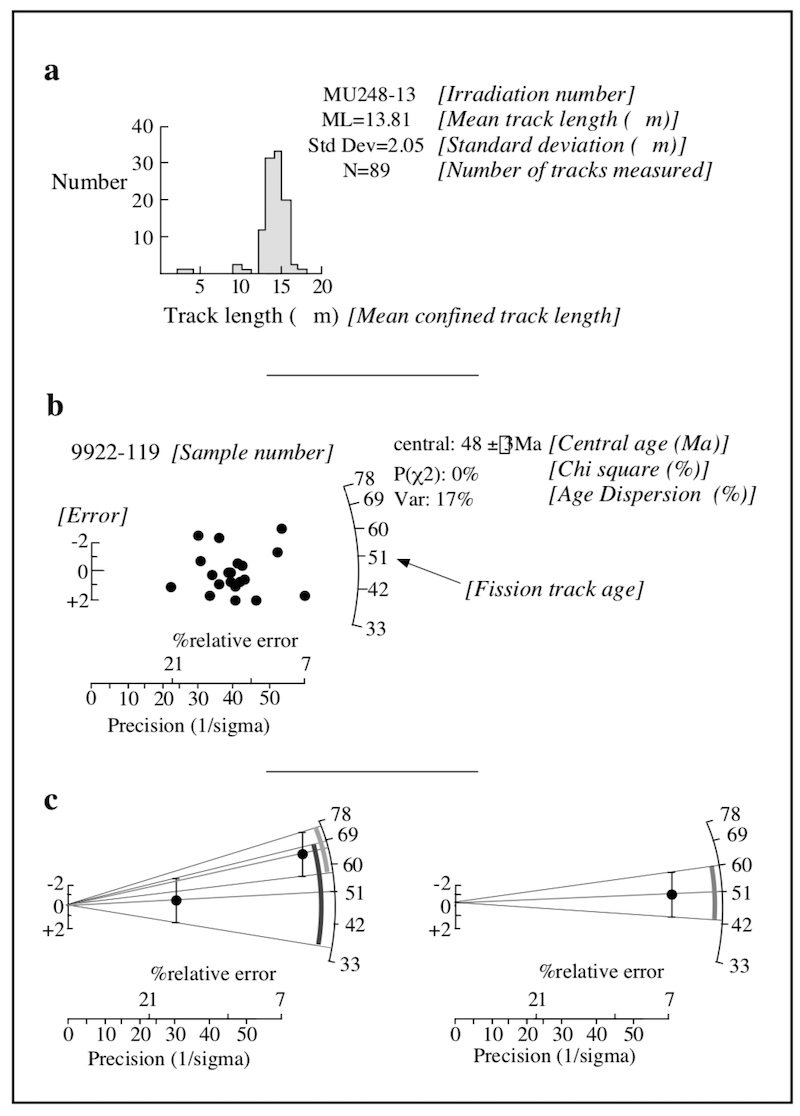
Figure 5.2
Graphical presentation of fission track age and length data. (a) shows confined track length data plotted as a histogram (normalised to 100 tracks), with 1μm length intervals. The mean length, standard deviation and number of tracks counted are displayed to the right of the graph. (b) shows fission track age information displayed as radial plots constructed using the method of Galbraith (1988, 1990). (c) demonstrates how to interpret the radial plot.

5.9 Fission Track Computation Software

Several computer programs are available which greatly assist in the calculation of fission track age results, assessment of errors and age dispersion, create radial plots, length and grain age distributions etc. Most fission track laboratories have some kind of software available for calculating fission trcak ages from raw data and many of these ar e in the public domain. Two excellent examples are MacTrack X for Mac OS X (Macintosh), available from the Melbourne Thermochronology Group on request, or Trackkey for Windows PC developed by Istvan Dunkl at Göttingen, Germany. Both these software packages are described in OnTrack 12(2), August 2002, p11-12). OnTrack is the newsletter of the international fission track dating community and is accessible online at the OnTrack Forum website. A number of useful software packages covering various aspects of fission track computation can also be accessed from the OnTrack Forum site, and also from Istvan Dunkl of the University of Göttingen, and Pieter Vermeesch of University College, London. Vermeesch (2009) describes his very useful cross-platform RadialPlotter software for constructing radial plots described in 5.7 above and available for download from here.

5.10 Thermal History Reconstruction and Interpretation

As explained in section 1, above, detailed consideration of the interpretation of fission track data and thermal history modelling is beyond the scope of this manual, but is discussed in detail by Gallagher at al. (1998) and Braun et al. (2006). Two particular software packages for this purpose are now in common use. These are HeFTy developed by Ricahrd Ketcham of the University of Texas at Austin (Ketcham 2005), and QTQt developed by Kerry Gallagher of the University of Rennes in France (Gallagher 2012). These software packages are available by contacting the authors directly. A number of these and other software tools for interpreting low-temperature thermohronology data are described by Ehlers et al (2005).